Big O Notation

Definition

An algorithm is a particular process for solving a problem, for performing an operation. Big O notation describes the performance (i.e. speed, efficiency) of an algorithm, that is, how fast an algorithm's execution time grows as the input size grows.

In Big O, how fast means how many steps, not how much time. This is known as runtime complexity. Big O measures how many steps an algorithm takes relative to how many input items are provided. In turn, space complexity is the amount of memory taken up by an algorithm, i.e. how much storage each item requires.

Why not use time for describing performance? Speed measurement in terms of time depends on the hardware that it is run on. It is impossible to say with certainty that an operation always takes, say, five seconds. A one-step algorithm may take five seconds on your computer, but take much longer on an older one, even if there is always one step to be executed. On the other hand, if Operation A takes five steps, and Operation B takes 500 steps, then Operation A will always be faster than Operation B on all computers. Therefore, we always focus on the number of steps.

We do not describe an algorithm as simply a "5-step algorithm" and another a "500-step algorithm", because the number of steps that an algorithm takes often depends on the size of the input. In a linear algorithm, if an array has five items, item-by-item search takes at most 5 steps, but if the array has 500 elements, item-by-item search takes at most 500 steps. To describe the performance of a linear algorithm, we say that it takes n steps for an n-sized input. Instead of focusing on units of time, Big O remains consistent by focusing on the number of steps that an algorithm takes.

In Big O, input size is always n, e.g. the number of elements in an array, or the number of nodes in a linked list, the number of bits in a data type, the number of entries in a hash table, etc. After determining what n means in terms of the input, you must determine how many steps are performed for each of the n input items. For n input items, an algorithm takes a relative number of steps.

For example, in a linear algorithm, if a step will be run on each of n input items, there will be n steps, the same number of steps. This is O(n) (pronounced "O of n") or linear time, where the time required to run the algorithm grows linearly with the size of the input. For n input items, a linear algorithm takes n steps: 2 items → 2 steps, 4 items → 4 steps. By contrast, for n input items, a quadratic algorithm takes n² steps: 2 items → 4 steps, 4 items → 16 steps; or consider O(1), which simply means that the algorithm takes one step regardless of the number of input items, as in reading from an array, which always takes one step regardless of how many items there are in the array. Other O(1) operations are insertion and deletion at the end of an array.

Approximation

In runtime complexity analysis, we always consider the worst-case scenario and take into account the highest order of n.

In the above example, if in addition to executing an operation on n items, we also have two initialization steps, it might seem more accurate to describe this algorithm as O(n + 2). Big O analysis, however, is concerned with the asymptotic running time: the limit of the running time as n gets very large.

The rationale for this approximation is that, when n is small, almost any algorithm will be fast. It's a reassurance—if linear, you know that it will never be slower than O(n) time. It is only when n becomes large that the differences between algorithms are noticeable. As n approaches infinity, the difference between n and n + 2 is insignificant, so the constant term + 2 can be safely ignored. In Big O, you eliminate all but the highest-order term, which is the term that is largest as n gets very large.

To determine the runtime complexity of an algorithm:

1. Identify the input, i.e. what n represents.
2. Express the number of operations that are dependent on the input size.
3. Eliminate all but the highest-order terms.
4. Remove all constant factors.

Because of approximation, an algorithm can be described as O(1) even if it takes more than one step: an algorithm can take three steps no matter how much large or small the input. In Big O, the difference is trivial. O(1) describes any algorithm that does not change its number of steps as the input grows.

Remember, Big O ignores constants, numbers that are not an exponent. O(n²/2) becomes O(n²), O(2n) becomes O(n), O(n/2) becomes O(n). Even O(100n), which is 100 times slower than O(n), becomes O(n).

While a 100-step algorithm is less efficient than a one-step algorithm, the fact that it is O(1) still makes it more efficient than any O(n) algorithm. For an array of fewer than one hundred elements, an O(n) algorithm can take fewer steps than an O(1) 100-step algorithm. At exactly one hundred elements, the two algorithms take the same number of steps (100). But here’s the key point: for all arrays greater than one hundred, the O(n) algorithm takes more steps. Because there will always be some amount of data in which the tides turn, and O(n) takes more steps from that point until infinity, O(n) is considered to be, on the whole, less efficient than O(1).

When two algorithms have the same Big O classification, this does not necessarily mean that both run at the same speed, e.g. bubble sort is twice as slow as selection sort but both are O(n²). Big O is good for comparing algorithms having different Big O classifications, but when two algorithms fall under the same classification, further analysis is required to determine which algorithm is more efficient.

Runtime Classification

Remember, Big O notation describes how many steps an algorithm takes based on input size. The fastest possible running time for any runtime analysis is O(1) (pronounced "O of 1") or constant time. An algorithm with constant running time always takes the same amount of time to execute, regardless of the input size. This is the ideal runtime for an algorithm, but it is rarely achievable. The performance of most algorithms depends on n, the size of the input. Those that run in constant, logarithmic and linear time are preferred.

Runtimes:

Runtime	Name	Example
O(1)	constant	one step outside loop
O(log n)	logarithmic	binary search
O(n)	linear	item-by-item search
O(n log n)	quasilinear	quicksort
O(n²)	quadratic	selection sort
O(2ⁿ)	exponential	certain recursive functions
O(n!)	factorial	recursive function inside loop

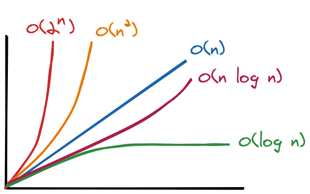
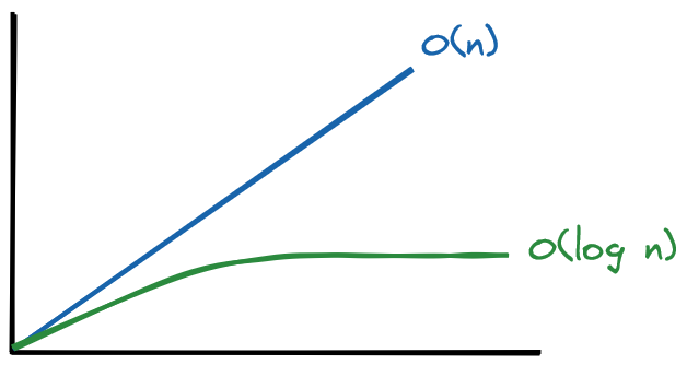
The runtimes here are ordered from best to worst performance: O(log n) (log time, reducing work by half in every step) is more efficient than O(n) (linear time, working item by item).

For example, for an array of five items, the maximum number of steps an item-by-item search would take is five. For an array of 500 items, the maximum number of steps an item-by-item search would take is 500. For n items in an array, linear search will take, at worst, n steps. Remember, we default to the worst-case scenario.

• O(1) describes an algorithm where the number of steps is independent from the input size. The speed of the algorithm is constant no matter how large the data.
• O(n) describes an algorithm where the number of steps increases in lockstep with the input size.
• O(log n) describes an algorithm that increases one step each time the input size is doubled. O(log n) is actually shorthand for O(log₂ n). For n input items, an O(log n) algorithm takes O(log₂ n) steps. For eight input items, the algorithm takes three steps, since log₂ 8 = 3.
• O(n²) describes an algorithm where the number of steps is the square of the input size. For n input items, the algorithm takes n² steps.

O(1)

public class Main() {
    public void log(int[] numbers) {
        System.out.println(numbers[0]);
    }
}

O(n)

public class Main() {
    public void log(int[] numbers) {
        for (int number : numbers)
            System.out.println(number);
        }
    }
}

O(n²)

public class Main() {
    public void log(int[] numbers) {
        for (int first : numbers) {
            for (int second : numbers) {
                System.out.println("hello");
            }
        }
    }
}

O(n³)

public class Main() {
    public void log(int[] numbers) {
        for (int first : numbers) {
            for (int second : numbers) {
                for (int third: numbers) {
                    System.out.println("hello");
            }
        }
    }
}

O(log n)

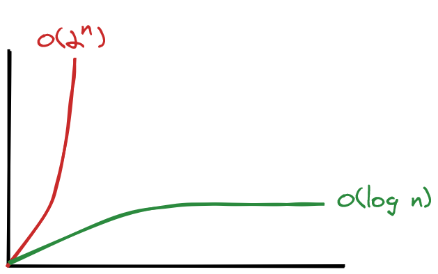
O(2ⁿ)

O(2ⁿ) (pronounced "O of 2 to the n") is exponential growth, the opposite of logarithmic growth.

Relationship with Data Structures

The organization of your data can significantly impact how fast your algorithm will run. Different data structures have different efficiencies with different operations.

An algorithm interacts with that data structure through four operations:

• Read: Looking up an item from a specific location in a data structure, e.g. providing an index to look up a value in an array.
• Search: Looking for the location of an item in a data structure, e.g. providing a value to looking for its index in an array, if it exists.
• Insert: Adding a value to the data structure, e.g. providing a value to be added to an array.
• Delete: Removing a value from the data structure, e.g. providing a value or index to be removed from an array.