Designing a geospatial search service

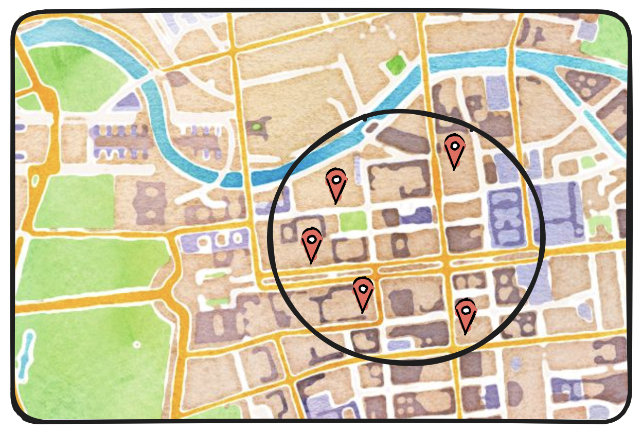
Behind many apps is a geospatial search service. Also known as proximity search, this allows users to find nearby shops, landmarks, people and other points of interest, often displayed as pins on a map. Google, Yelp, WhatsApp, Uber and Tinder all rely on geospatial search to power their map navigation features. Discovering nearby spots is one of the most common use cases for location-based apps.

How might we go about implementing a proximity service? That is, given a pair of coordinates and a radius, how do we implement a service to find all nearby points of interest? And in doing so, how do we keep our search both efficient and scalable? What are our options and what are the tradeoffs between them?

Let's explore what it takes to design a geospatial search service.

Framing the design

Functionally, we must satisfy one requirement: given a user's current location and a search radius, return all nearby points of interest. Note that our search service will support, and be supported by, a second service to manage point-of-interest data, allowing users to create, update, and delete points of interest; these changes need not be reflected in real time. While we will focus on geospatial search, we should be mindful of the point-of-interest management service we will work in tandem with.

Non-functionally, our geospatial search must offer:

• Speed. The search service should return nearby points of interest quickly.
• Availability. Our architecture should not hinge on a single point of failure.
• Scalability. We should accommodate traffic spikes during peak hours.

A starting point for our design might look like this:

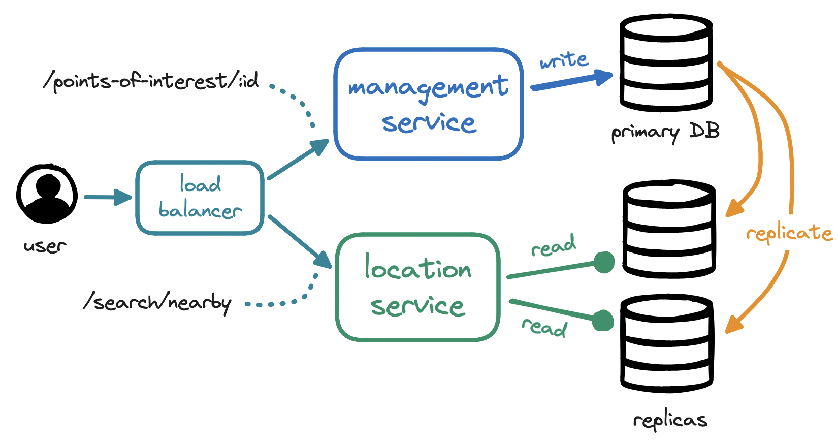
The term "point of interest" (PoI) refers to any place of relevance to users, such as restaurants and hotels, based on our business needs. The management service is tasked with mutating point-of-interest data, which is unlikely to change frequently, so this is a write-only service expecting a low request volume.

By contrast, the location service is read-heavy and expects a high request volume, especially during peak hours in densely populated areas. For higher scalability and availability, our location service...

• will remain stateless so we can scale it out horizontally, adding and removing servers in line with traffic load, and
• will interface with a database cluster containing a primary database for writes and multiple read replicas.

The location service has a single responsibility: finding points of interest within a radius from the user's position. Making this search efficient will be the crux of our discussion.

Geospatial search algorithms

To find points of interest within a radius, our first instinct might be:

SELECT * FROM points_of_interest
WHERE (
	lat BETWEEN :user_lat - :radius
	    AND :user_lat + :radius
)
AND (
	long BETWEEN :user_long - :radius
	     AND :user_long + :radius
);

B-trees in relational DBs are hierarchical—each level narrows down the search space. For range queries, especially over multiple columns, we must traverse several levels to find all values in the range, meaning that this lookup will lead to a full table scan. Even with indices on latitude and longitude, we cannot speed up this query by much, as we still need to intersect two sets of results.

Our lookup is conditioned by our two-dimensional data. We could keep pushing in this direction for incremental improvements, e.g. with a composite index, but this might also be a good time to rethink our approach. How can we simplify this lookup? Is there a solution to combine our two columns into one?

Geohashing

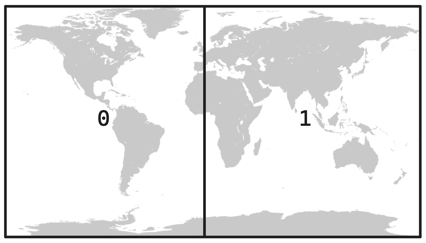
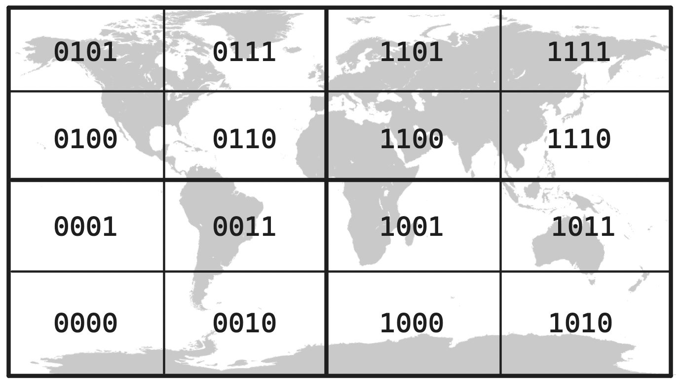
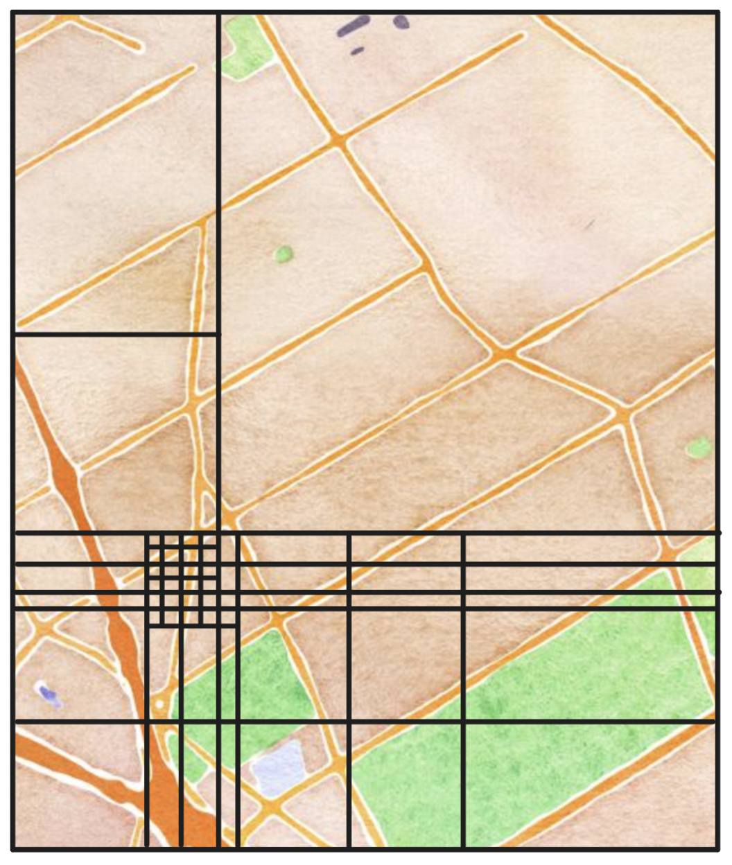
One such solution is geohashing, which encodes latitude and longitude into a single value. To achieve this, we first split the world along the prime meridian, i.e. into the Western and Eastern hemispheres, labeling each half in binary:

Next we split each hemisphere into halves and label them, prefixing each label with that of the original hemisphere, starting from the bottom:

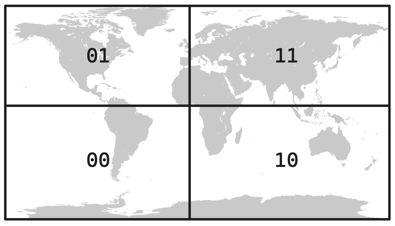
This process is recursive: we keep subdividing each labeled quadrant into smaller and smaller ones. Each of these labels is known as a geohash—the longer the geohash, the smaller the section of the world it refers to. We are naming increasingly granular sections in a grid of the world, instead of relying on a pair of coordinates.

As grid sections become smaller and smaller, labels become longer and longer. For example, the label 11110000110001101101011000000111011 refers to a public square in the heart of Berlin. For convenience, we typically encode geohashes in base32, which compresses this binary label into a handier u33dc1r. Geohash precision can range from the size of the world to the order of centimeters.

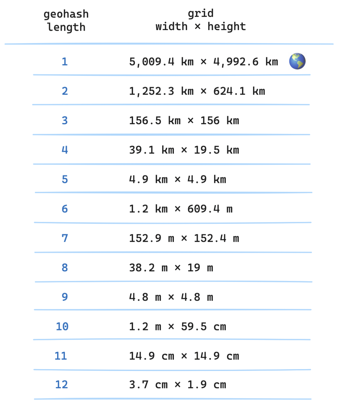
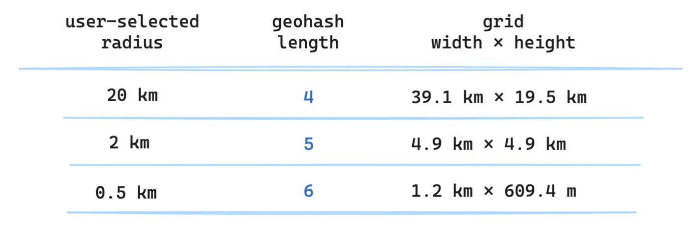
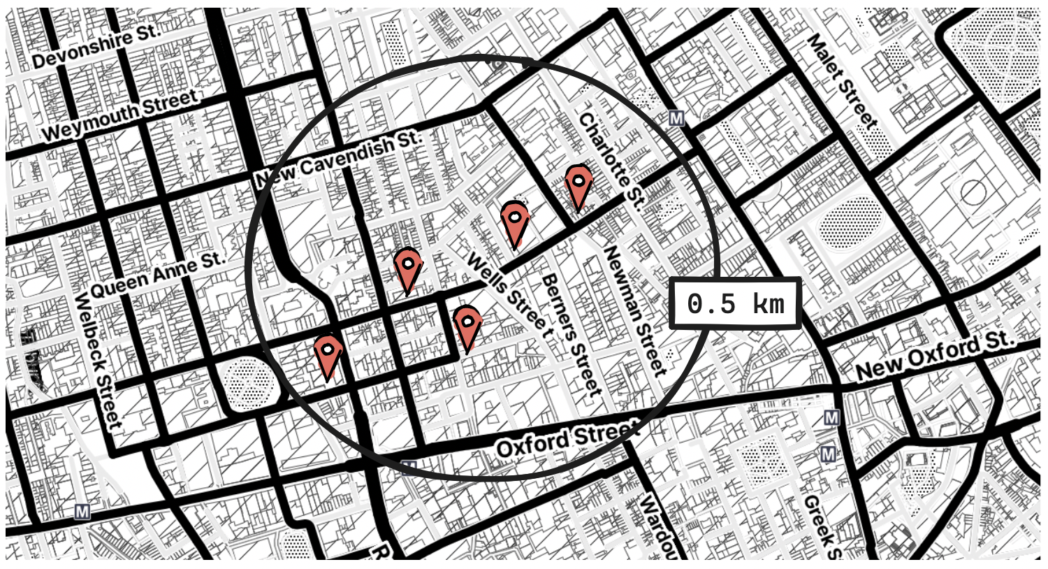
How does this relate to our problem? We need to find all points of interest within a radius, i.e. we need to find a geohash that labels an area that covers the entire circle drawn by the radius. This means that the radius will dictate our geohash precision, which in turn means that only a subset of all these precisions is practical for our purposes. Realistically, this is likely to be a geohash of length four, five, or six.

Is geohashing the solution? Suppose we were to store a geohash for each point of interest. Given the geohash for the user's location, could we then query by matching it to the initial characters in the geohash for each point of interest?

SELECT * FROM geohashes WHERE geohash LIKE '8n8zn%';

Not quite. Geohashes have a useful property: the longer the shared prefix between two geohashes, the closer their locations. For instance, the geohashes 8n8zn3 and 8n8zn9 are adjacent, sharing all characters but the last.

But the opposite is not always true: close locations do not necessarily have similar prefixes. Two locations that are close to each other may have no shared prefix at all, e.g. adjacent locations on each side of the equator. Further, two locations can be right next to each other and still be assigned different geohashes.

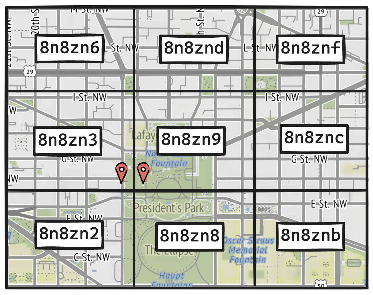
To address these edge cases, we can fetch all points of interest in the user's geohash and also in its eight neighbors. Since a geohash can be computed in constant time, the retrieval will remain efficient, but pay attention to the tradeoff between inclusion and precision. We will be querying for slightly more than the rectangular area that covers the size of the circle around the user's location.

Quadtree

This tradeoff might give us pause. If geohashing operates on uniform quadrants but may lead to suboptimal queries, we might start wondering about more precise options, of which the quadtree is a popular one.

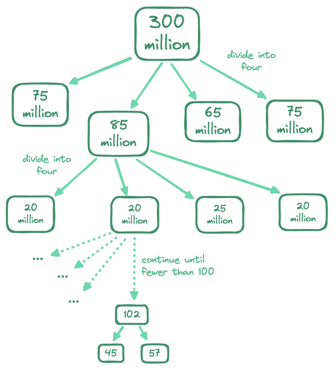
Imagine again we were to recursively partition the world. But this time, instead of the base case being the smallest grid section, let's keep subdividing until every grid section meets the condition of containing at most 100 points of interest. This way, we will end up with grid sections of varying sizes, that is, we will have subdivided the world based on the density of points of interest, producing larger sections for sparsely populated areas and smaller sections for denser ones.

In essence, a quadtree is a tree where the root represents the entire world and each non-leaf node has four children. To find all locations within a radius, we start at the root and traverse the tree until we reach the target leaf node holding the user's location. If the target leaf node has the desired number of points of interest, we return the node, else we add locations from its siblings until reaching the threshold.

The implementation details of the quadtree are beyond the scope of this discussion, but we should keep its operational implications in mind. Notably, a quadtree is an in‑memory data structure, built during server startup. While its memory consumption is low enough, it will take a few minutes to build—during this time, a server cannot serve traffic, so we should only rebuild a subset of quadtrees at a time.

Also, we need to keep quadtrees in sync with additions, updates, and deletions of points of interest. The simplest here would be to rebuild all quadtrees in small batches across the cluster on a nightly basis, since the requirements do not call for changes to be reflected in real time. If it ever came to this, we would need to edit quadtrees on the fly—a tough proposition that would involve ensuring safe concurrent access to the quadtrees and rebalancing them where needed.

Data modeling for geohashing

Geohashes and quadtrees are both widely adopted, but the quadtree's operational implications might lead us to lean on geohashing as the simpler of the two. Assuming we have settled on geohashing, how should we model our data?

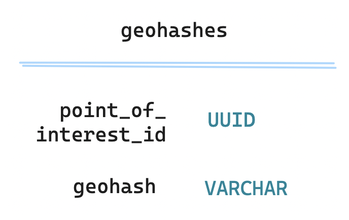
The points_of_interest table should be straightforward:

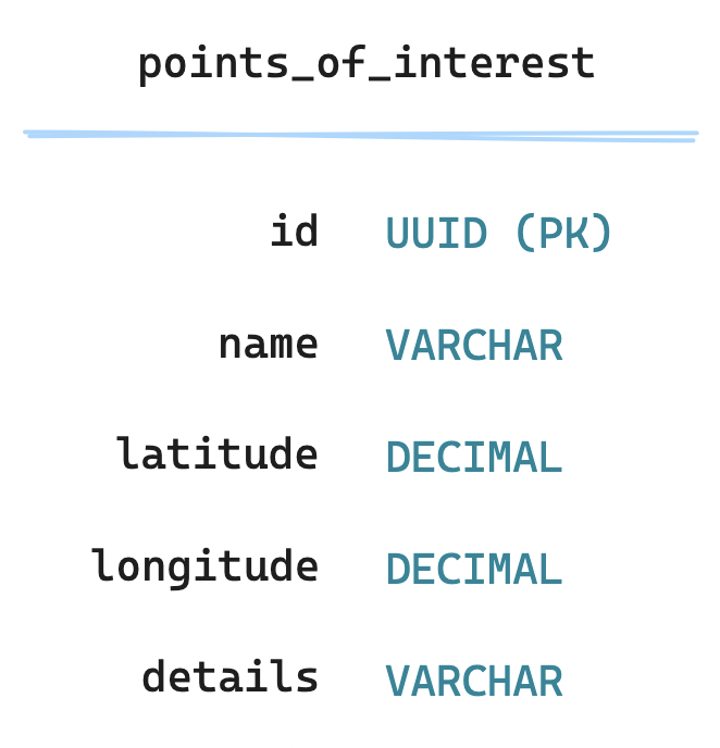
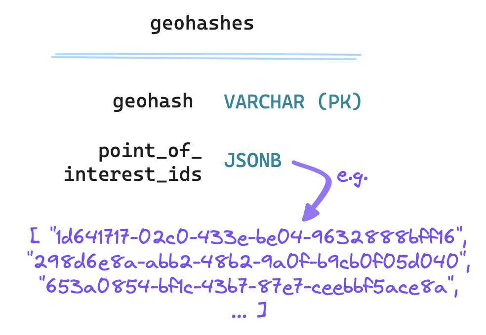
But how should we map them to geohashes? One approach could be to denormalize: for each geohash, store a JSON array of IDs for points of interest, i.e. all the locations inside the area labeled by the geohash. This allows us to retrieve all points of interest for a geohash in constant time. But editing this array is a costly operation, especially for densely populated geohashes; we should also be careful to dedupe on insertion and lock rows to prevent concurrent writes.

The opposite approach would be to normalize: ensuring each row holds a single geohash and a single point of interest, with a composite key made up of both.

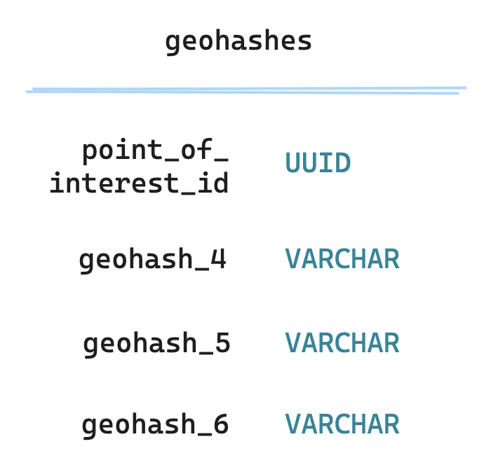
In exchange for more space and slightly slower retrieval, normalization here makes for much simpler additions, removals and updates, no row-locking needed. This option also lends itself to optimization. For example, since we expect to match on geohashes of multiple precisions, and since the LIKE operator is not index-friendly, we could store geohashes of different lengths and match on them specifically, at the cost of even more space, if we needed to speed up retrieval even further.

Going further

Zooming back out to our high-level design, let's trace the lifecycle of a request:

1. The user navigates to a map tile and triggers a request for nearby points of interest, informing the user's coordinates and a search radius.
2. Our load balancer receives and forwards the request to the location service.
3. The location service converts the user's coordinates into a geohash.
4. The location service queries the geohashes table (on a read-only replica) for all IDs of points of interest matching as much of the geohash as required by the search radius. Alternatively, we match on the entire geohash if we have laid out one column per geohash length.
5. The geohash service then queries the points_of_interest table for all entries matching the IDs obtained from the query to the geohashes table.
6. The location service finally returns the nearby points of interest, to be displayed to the client as pins on a map.

To implement this lifecycle, we have discussed two algorithms fundamental to geospatial search, i.e. geohashing and quadtrees, digging into their working principles as well as some of their strengths, limitations, operational implications, and data modeling considerations as they apply to our design.

To go further, consider:

• how to optimize geospatial searches for a user in motion,
• how to devise a caching strategy for densely populated areas,
• how to fetch all neighbors of a geohash to account for its edge cases,
• how to auto-expand the search radius if no points of interest are found, and
• when to bring in a modern option like Google's S2 geometry library.

Geospatial search is an area of very active research, with many practical applications beyond the discovery of nearby locations—such as geofencing, route planning, mobility prediction, and real-time navigation. Designing a geospatial search service can be an accessible point of entry to this rapidly evolving field.